Tej Bade, tbade12@berkeley.edu

Back to Portfolio

Project 1: Image Quilting

In this project, we implement texture synthesis and texture transfer. Texture synthesis involves taking an image of a texture and creating an image of a different size that has the same patterns. Texture transfer involves taking an object and applying a texture from a different image to it. This project follows the paper here.

Randomly Sampled Texture

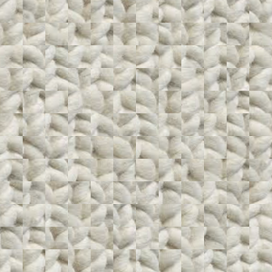
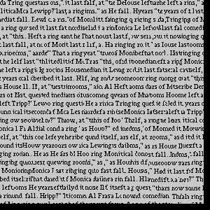
We use the following texture image.

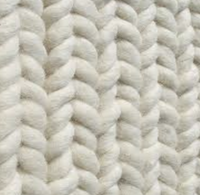
A naive approach to texture synthesis is randomly sampling square patches from a source image and concatenating them row by row until we fill the output image. Shown below is the original texture image and the output image with random sampling.

Overlapping Patches

To create a better a texture, we can choose patches that align well with existing patches and overlap them. We start by randomly sampling a patch and placing it in the top left of our quilt. Then, we find the patches that, when placed on top of the adjacent patches, minimizes the sum of squared differences (SSD) in the overlapping regions. We randomly choose a patch out of the $tol$ best patches and place it in the output image. We do this row by row until we get the final image. Shown below is the original image and the image produced by this method.

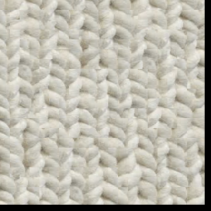
Notice that we can still see the edge artifacts if we look at the image closely.

Seam Finding

Instead of overlapping the patches by directly placing a patch onto an existing one, we can try to find an optimal path across the overlapped region that acts as a boundary for which patch to take the final pixel from. To do this we leverage dynamic programming and keep track of the minimum total error along the path. We define the error $e_{i,j}$ of a pixel location $(i, j)$ as the squared difference of the pixels in each patch. Let $E_{i,j}$ be the minimum path ending at $(i, j)$. Then, we can calculate the path by

$E_{i, j} = e_{i, j} + \min(E_{i-1, j-1}, E_{i-1, j}, E_{i-1, j+1})$

We can set this path as our boundary and overlap the patches. The original image and output image are shown below.

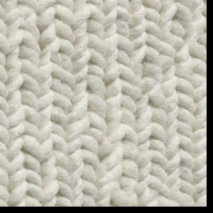
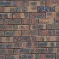
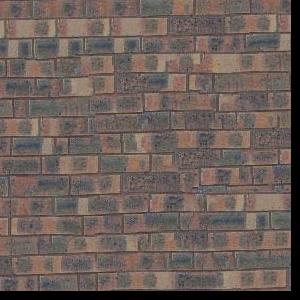
Here are results for two other textures.

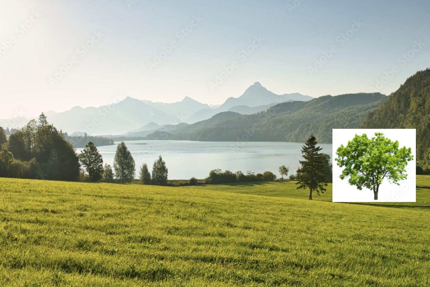
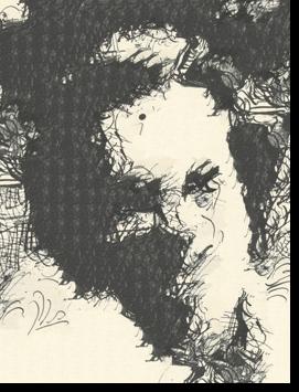
Texture Transfer

Now we attempt to give an object the texture of another image. We add another term to our cost function that tells how well the sampled patch matches the structure of the patch in the output image. I used blurred luminance values for the source and target guidance images and used the sum of squared differences between the sampled guidance patch and target guidance patch.

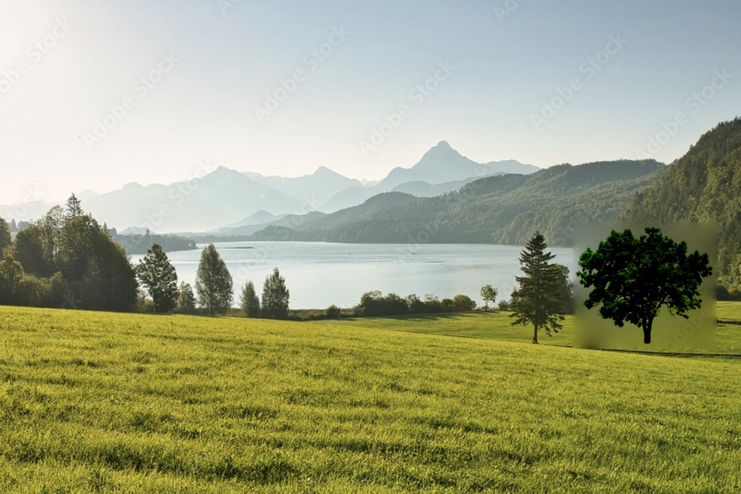
The following two images are .tiff images that were converted to .jpg for the purpose of showing them on this webpage.

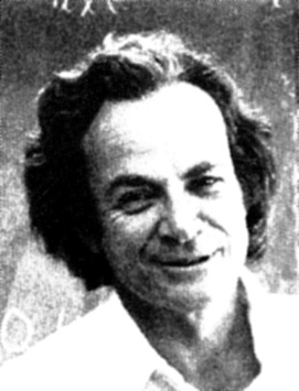
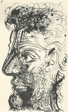
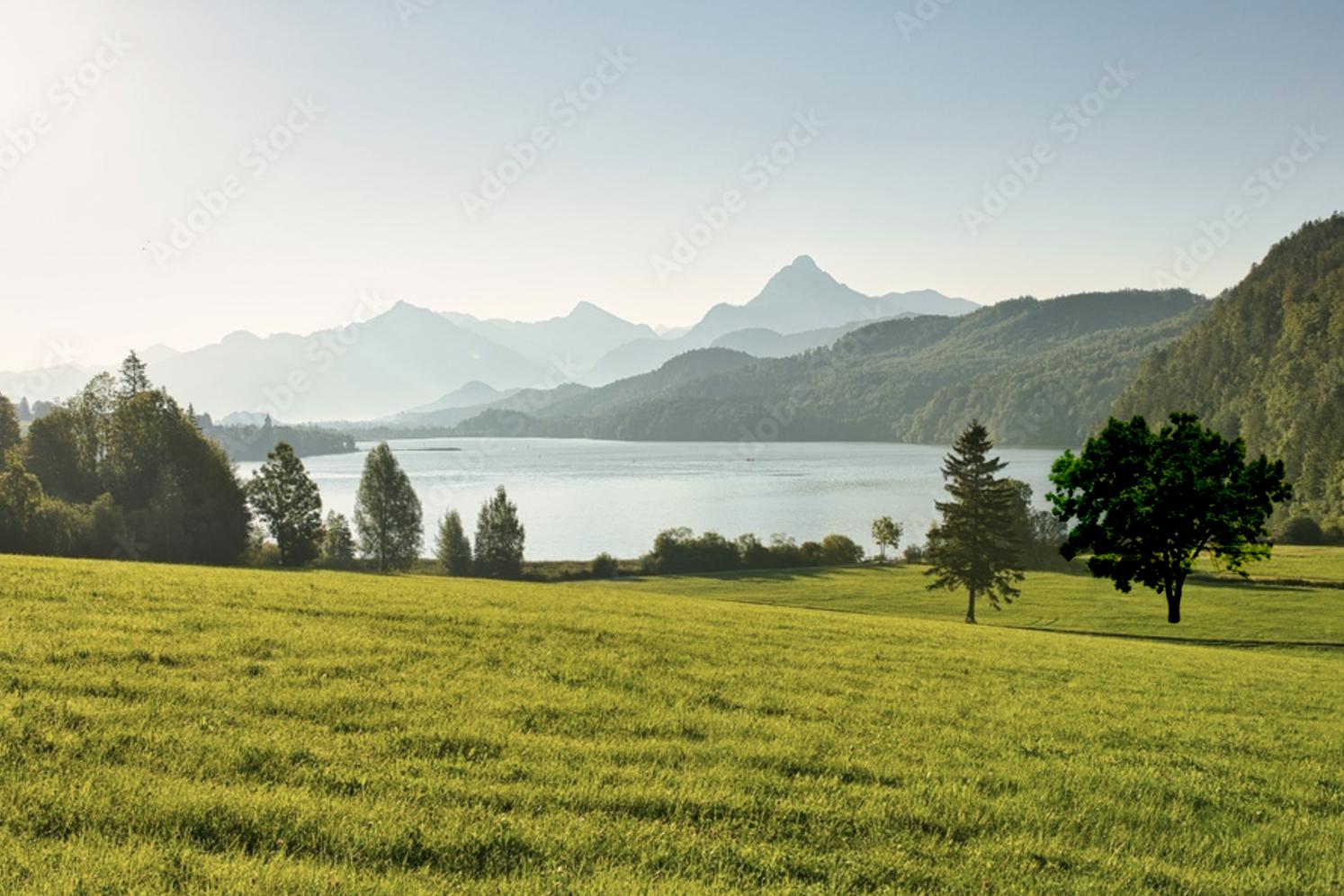
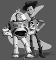
Using the .tiff images, I created the image with the texture transferred. It is shown below.

Project 2: Gradient Domain Fusion

In this project, we implement gradient domain fusion. This involves blending an object into another image using gradients across the images. I used the starter code and utility functions that were given here.

Part 1: Toy Problem

For this part, we take an image and reconstruct it using gradients. We use the test image below.

For each pixel $i$ we want to minimize $((v(x+1, y)-v(x, y)) - (s(x+1, y) - s(x, y))^2$, which ensures that the x-gradients of $v$ match the x-gradients of $s$. Similarly, we want to minimize $((v(x,y+1)-v(x,y)) - (s(x,y+1)-s(x,y)))^2$ to ensure the y-gradients match. Finally, we start with a pixel intensity of the source image in the upper left by adding one more minimization: $(v(0,0)-s(0,0))^2$. We treat the reconstructed image as a vector and solve for it as a least squares problem. This gives us the reconstructed image below.

Part 2: Poisson Blending

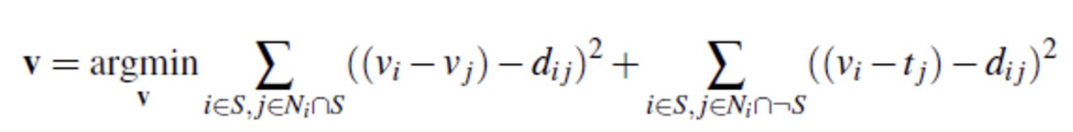
We can use the basic logic behind the Toy Problem to blend an object into another. If we let $s, S, t,$ and $v$ be the source image, source region (part of the source image that contains the object we blend into the target image), target image, and target region, we can use the equation below to solve for $v$.

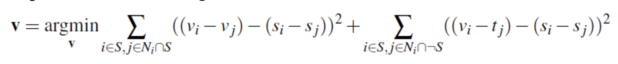
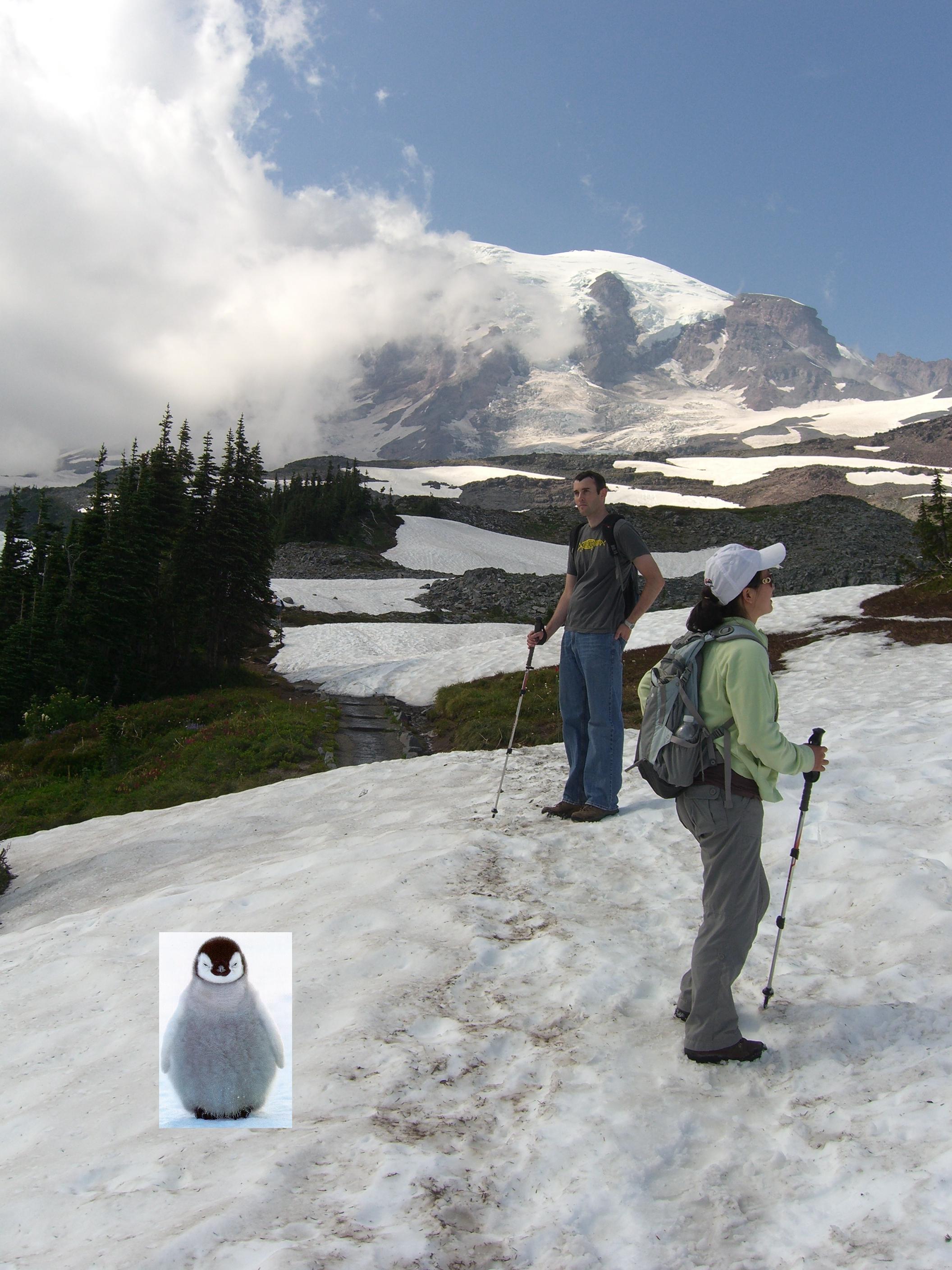
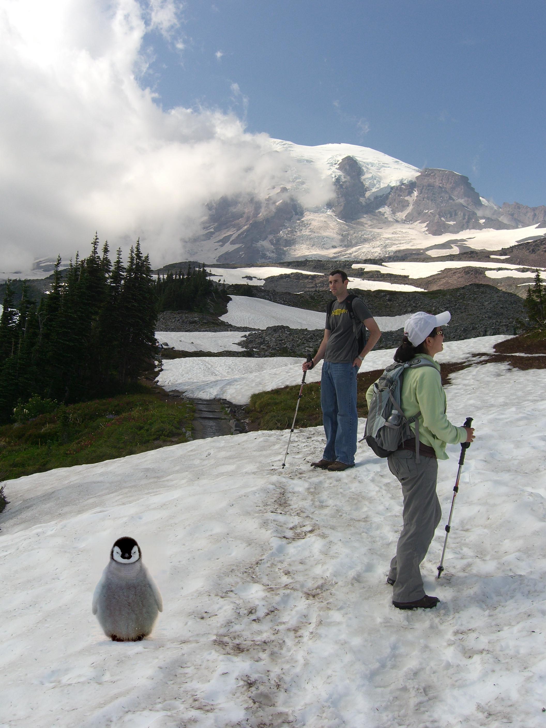
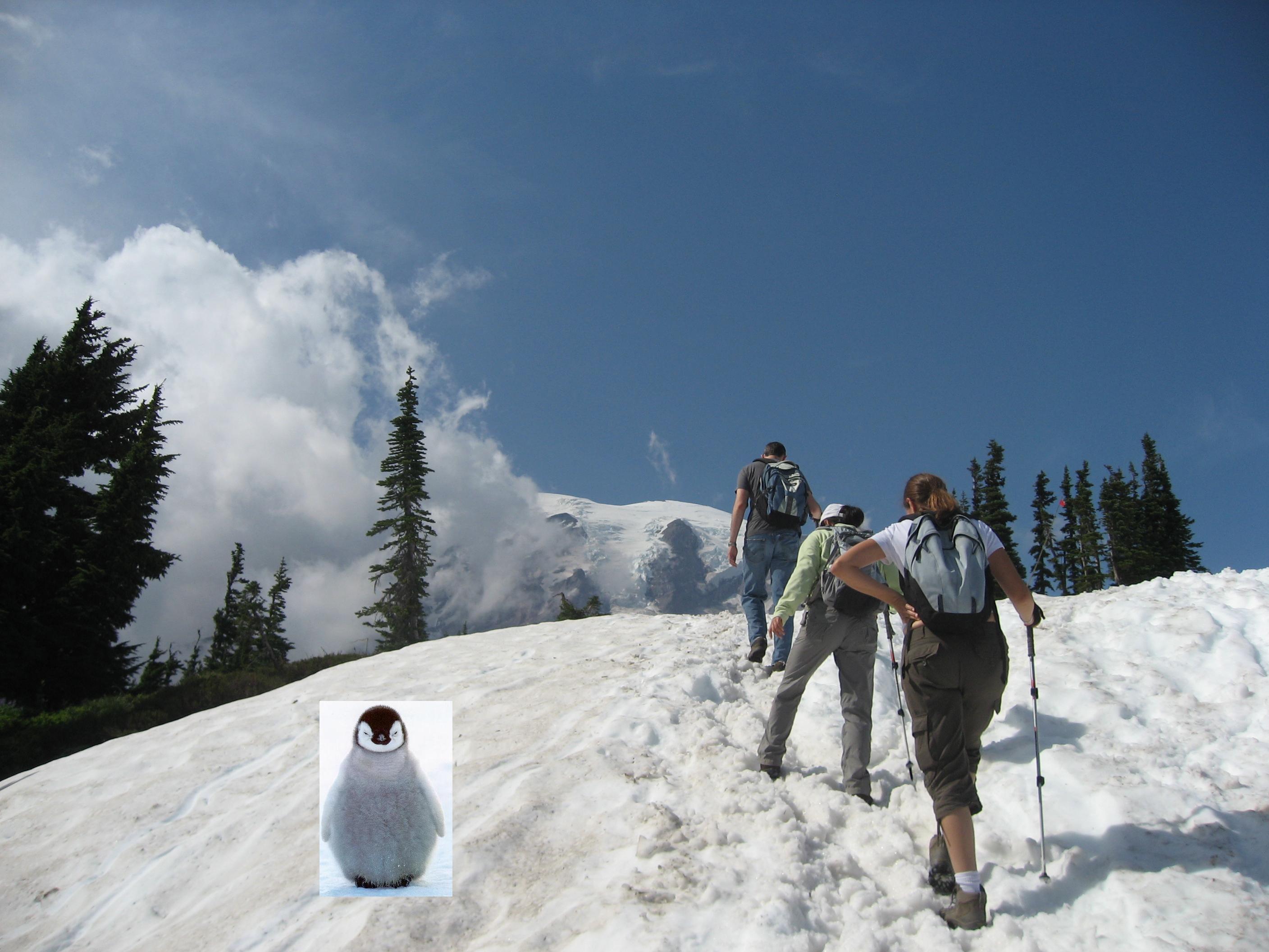
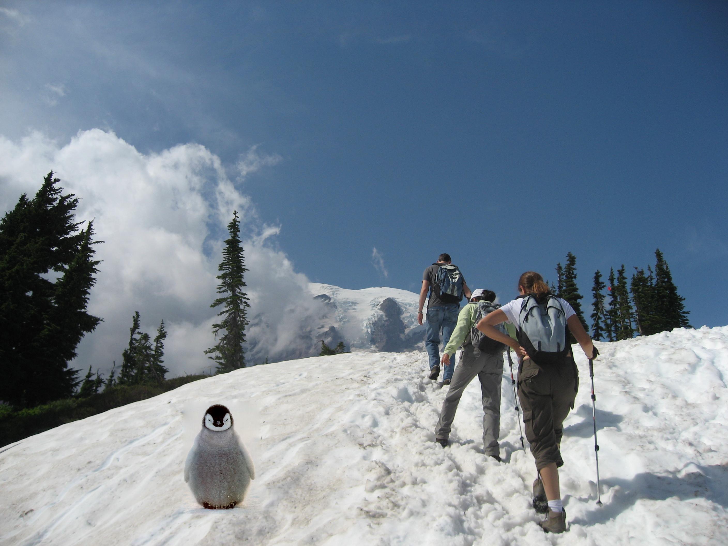
$N_i$ refers to four neighbors of pixel $i.$ I first blended an image of a penguin onto a snow slope using this method. The left image is just the penguin (source region) placed onto the slope and the right image is the blended image.

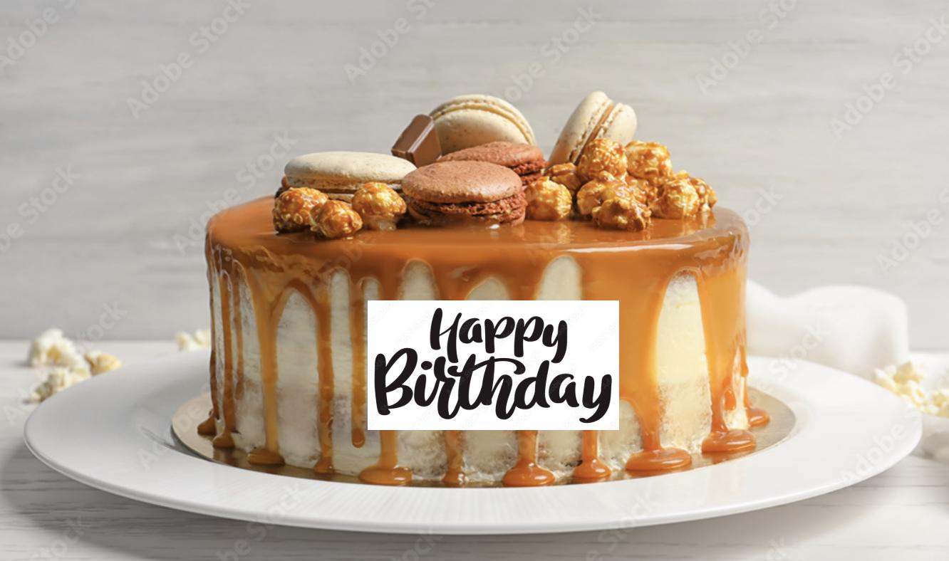
Here are two other examples:

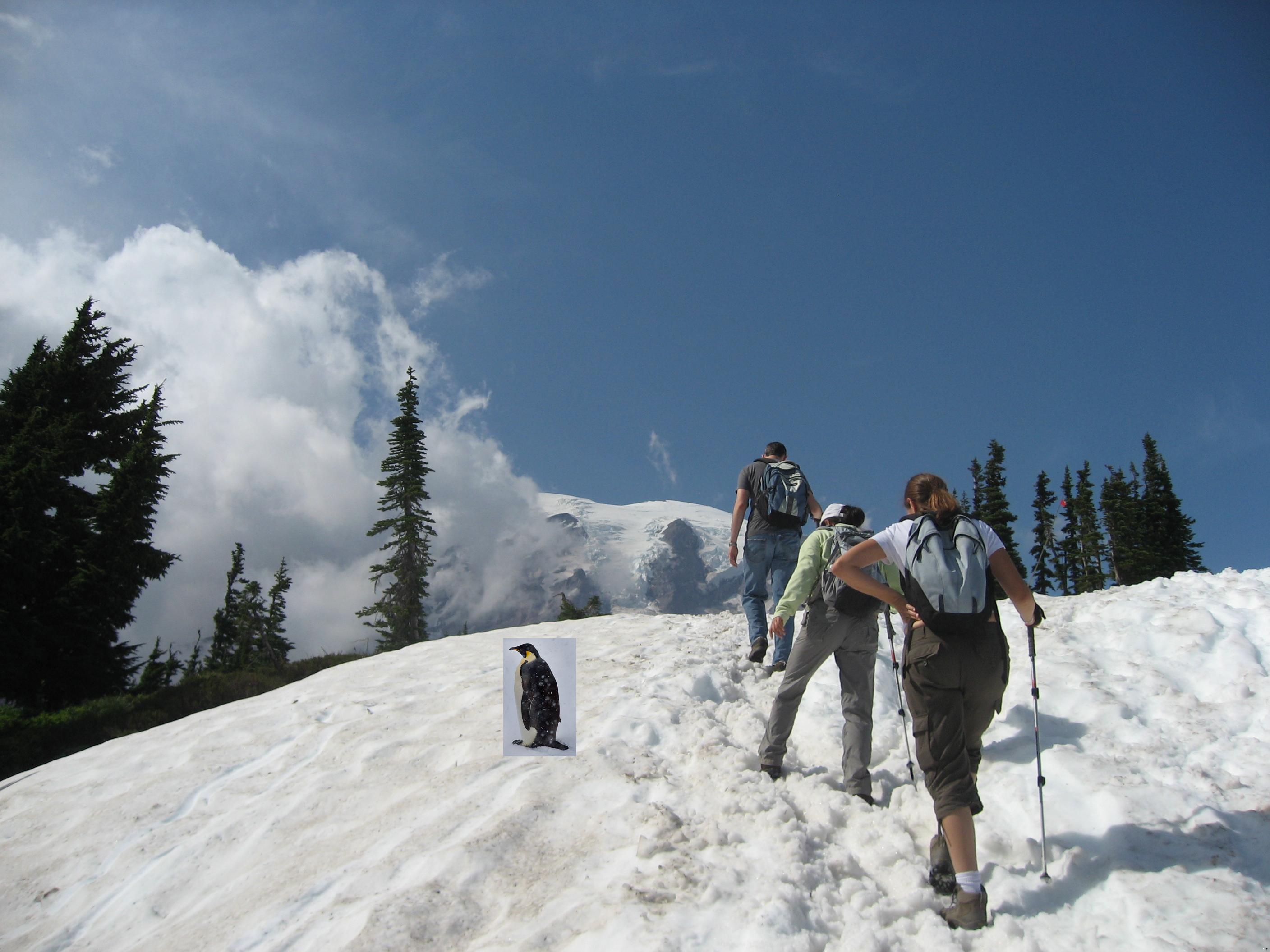
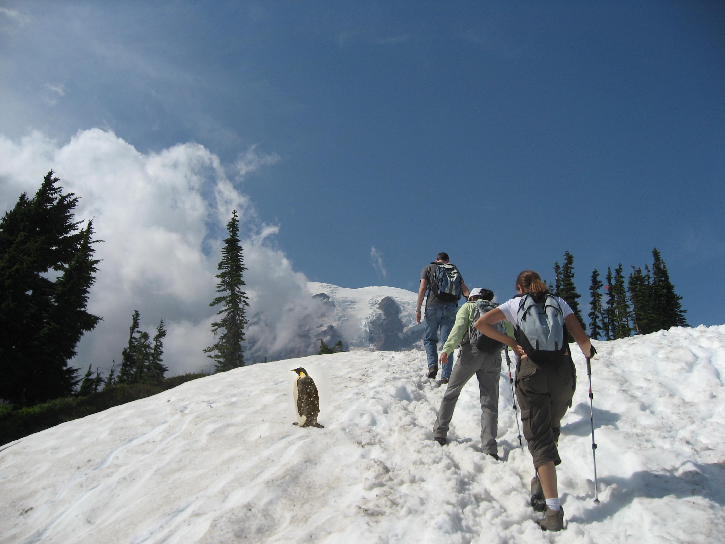
I think the blending works well for these examples because the target regions that the penguins are being blended into do not have dramatic color changes. In the “Mixed Gradients” section, we see the case where Poisson blending does not work well.

Bells and Whistles

Mixed Gradients

We can modify our method above using the following equation.

Whichever of $s_i$$-s_j$ and $t_i - t_j$ has the larger absolute value is set to $d_{ij}$.

The target image I used with the source region pasted on it is shown below.

I then blended the images with both the regular poisson blending and mixed gradient methods.

It seems that we can see the source region containing the object much more easily with Poisson blending than with mixed gradients. Another example is presented below.